- Thu 20 July 2017
- posts
- Michael Campbell
- #data-science, #data-analysis, #UCI
Finding spam in Youtube comments.
Spam has been around since the beginning of the Internet. The use of spam over a network, in fact, stretches all the way back to 1884 when wealthy Americans were sent unsolicited investment offers over the telegraph[1]. In more modern times, the first appearance of modern email spam occured on ARPANET, a military precursor to the Internet, when 'a man named Gary Turk sent an e-mail solicitation to 400 people, advertising his line of new computers'[1].
In this notebook we will consider the problem of finding spam in Youtube comments. Spam in Youtube comments is a slightly different task then spam in email. Youtube comments tend to be short, often less than five words, and a spam email may simply contain the name of the website domain. However, it is quite easy to construct a machine learning model to classify comments as spam or ham (not spam) with a high degree of accuracy.
For a training and test set, I will use the spam database found on the UCI machine learning repository. There are several different types of algorithms which can be used to classify spam; however, in this notebook, I will compare three specific models:
- Logistic Regression
- Naive Bayes Classifier
- Recurrent Neural Networks
While simple, the logistic regression performs quite well at classifying emails as spam or ham, and manages to achieve an f1 score (a common metric to evaluate models) of ~.9 on the test set. The neural network and naive Bayes classifiers perform well, though not as good as the logistic regression algorithm, with f1 scores of .84 and .85 on the test set.
Table of Contents
%matplotlib inline
import matplotlib.pyplot as plt
import numpy as np
import pandas as pd
import tensorflow as tf
import re
import os
Data analysis, preprocessing 
The UCI machine learning repository contains a dataset consisting of comments from five youtube videos that are classified as spam or not spam[2]. These are stored as csv files, which will be loaded into a list of dataframes. The classification data is stored as the class field, where comments with a class value of 1 are considered spam and comments with a class value of 0 are ham.
file_names = ['Youtube01-Psy.csv','Youtube02-KatyPerry.csv','Youtube03-LMFAO.csv',
              'Youtube04-Eminem.csv','Youtube05-Shakira.csv']
filepath = 'c:/users/michael/documents/github_data/data'
dataframes = [pd.read_csv(os.path.join(filepath,file_name)) for file_name in file_names]
dataframes[0].head(3)
To get a better sense of the data, I will print out the content for several reviews.
for content in dataframes[0].CONTENT[14:20]:
    print(content)
Cleaning the data 
There are several features unnecessary columns such as COMMENT_ID, AUTHOR, and DATE. Within content, there are a lot of web links. To make it easier to identify weblinks, I will substitute in the word WEBLINK for every instance of a URL. The character /ufeff is also present in the file, which is most likely due to improperly decoding utf-16 as utf-8. I will also define a function to remove this.
def format_sentence(s):
    ret_sent = re.sub('http\S+','WEBLINK',s)
    ret_sent = re.sub(r'\\ufeff','',ret_sent)
    return ret_sent
Splitting the data into test and training sets 
So I will be able to test the data, I will split the data into a test and training set. The training set will be used along with cross validation to select the best model. The model will then be evaluated by testing it on the test dataset.
from sklearn.model_selection import train_test_split
data = pd.concat(dataframes).reset_index(drop=True)
X_train,X_test,y_train,y_test = train_test_split(data.CONTENT,data.CLASS)
Turning the sentences into usable vectors 
In order to use a machine learning algorithm to predict from a collection of sentences, it's necessary to use a mapping that will associate every word, and every sentence with a vector that can then be feed into the machine learning algorithm. The simplest way to do this is to use the bag of words model, or create vectors by finding the term-frequency inverse-document-frequency of each sentence.
Bag of words Model 
I will first use a bag of words model to turn each sentence into a unique vector. The bag of words model is simply turning each word into a basis vector in a Hilbert space. To form a vector for the words, I simply add the vectors for each word for each sentence. Thus each sentence will be transformed into a vector that can be added to a machine learning model. In this model, given the sentences
- 'I ran to the store',
- 'I ran across town',
- 'I ran to work and to home',
the basis vectors would correspond to the words ('I','ran','to','the','store','across','town','work','and','home'). The sentences would then be encoded as the vectors
- (1,1,1,1,1,0,0,0,0,0)
- (1,1,0,0,0,1,1,0,0,0)
- (1,1,2,0,0,0,0,1,1,1)
However, this model can still be improved. For example, the words 'the', 'a', and 'of' occur so often that they are unlikely to help us classify comments. The words that are common enough that they do not aid in distinguishing sentences are called stopwords. Another limitation is that our implementation above would classify 'bag' and 'bags' as two different words. For this bag-of-words model, the verb tense or the s at the end of a word doesn't significantly affect the meaning of the word in the sentence. In order to reflect this, I will associate every word with a stem, that represents its most basic feature. ie. 'run', 'running', and 'runs' might all be replaced by the same word 'ru'. To achieve this, I will use a porter stemmer, which is found in the nltk.
Another limitation is that words that only occur once during the document do not add any predictive power. Because of this, I will ignore any words that occur less than five times.
TFIDF 
The bag of word vectors can be improved using one more feature which mapping each count in a vector to its term frequency/inverse document frequency. A term which appears five times in one comment is likely important. This is referred to as the term frequency. However, if that same term appears five times in every comment, then it is likely a commonly used word, 'the' for example. This is the document frequency The term frequency/inverse document frequency is simply the ratio of the term frequency to the inverse document frequency. The precise definition is to let the number of times a term $t$ appears in document $d$ be $tf(t,d)$. Let $n_d$ be the total number of documents in the corpus, and let $df(t)$ be the number of documents containing term $t$. Then the term-frequency calculated in the sklearn TfidfVectorizer is $tfidf(t,d)$ is $$tfidf(t,d) = tf(t,d)\cdot\text{log}\left(\frac{1+n_d}{1+df(t)}+1\right)$$ (Note, this differs slightly from the tfidf given in textbooks). The resulting vectors are then normalized.
from sklearn.feature_extraction.text import CountVectorizer
from sklearn.feature_extraction.text import TfidfVectorizer
import nltk
from nltk.stem.porter import PorterStemmer
def port_tokenizer(text):
    words = re.split(r'\s+',text.lower())
    ps = PorterStemmer()
    return [ps.stem(word) for word in words if not word in nltk.corpus.stopwords.words('english') and word]
count_vect = CountVectorizer(preprocessor=format_sentence,tokenizer=port_tokenizer,min_df=5)
tfidf_vect = TfidfVectorizer(preprocessor=format_sentence,tokenizer=port_tokenizer,min_df=5)
X_train_bow = count_vect.fit_transform(X_train)
X_train_tfidf = tfidf_vect.fit_transform(X_train)
print(X_train_bow.shape)
Predicting spam vs ham 
Model evaluation criteria 
Now that I have transformed the sentences into feature vectors, I will create and compare several machine learning algorithms to predict whether or not a given word will be spam. Since in the real world, spam occurs infrequently compared to ham, a classifier which simply predicted everything as ham would have a high accuracy. Because of this, accuracy is not the prefered way to measure the performance of a spam classifier. Instead I will use a combination of precision and recall
- precision: The number of true positives divided by the number of elements predicted to be true (true and false positives)
- recall: The number of true positives divided by the number of all positives (true positives and false negatives) Since I want to maximize both of these at the same time, I will use the f1-score, which is defined as the product of precision and recall, divided by their mean. $$f_1 = \frac{\text{precision}\cdot\text{recall}}{(\text{precision}+\text{recall})/2}$$
from sklearn.metrics import f1_score
Logistic Regression 
One of the simplist models that could be used to predict spam would be a logistic regression. The logistic regression model will choose its parameters via a grid search which will alter the regularization term C. I will also try using both the bag of words, and the tfidf vectors.
from sklearn.linear_model import LogisticRegression
from sklearn.grid_search import GridSearchCV
course_params = {'C':[2**x for x in range(-6,15,2)]}
gs = GridSearchCV(LogisticRegression(class_weight='balanced'),course_params,n_jobs=-1,cv=5,scoring='f1')
gs.fit(X_train_bow,y_train)
fine_params = {'C':[gs.best_params_['C']*(2**x) for x in np.arange(-1.75,2,.25)]}
gs = GridSearchCV(LogisticRegression(class_weight='balanced'),fine_params,n_jobs=-1,cv=5,scoring='f1')
gs.fit(X_train_bow,y_train)
print(gs.best_params_)
print(gs.best_score_)
sample_sizes = range(100,1000,10)
train_bow,test_bow = list(),list()
lr_bow = LogisticRegression(class_weight='balanced',C=gs.best_params_['C'])
for sample_size in sample_sizes:
    xs,ys= X_train[:sample_size],y_train[:sample_size]
    count_vect = CountVectorizer(preprocessor=format_sentence,tokenizer=port_tokenizer)
    xs_bow = count_vect.fit_transform(xs)
    xs_train,xs_test,ys_train,ys_test = train_test_split(xs_bow,ys)
    lr_bow.fit(xs_train,ys_train)
    train_bow.append(f1_score(lr_bow.predict(xs_train),ys_train))
    test_bow.append(f1_score(lr_bow.predict(xs_test),ys_test))
plt.plot(sample_sizes,train_bow,c='r',label='training set')
plt.plot(sample_sizes,test_bow,c='b',label='test set')
plt.xlabel('no of samples')
plt.ylabel('f1 score')
plt.title('Bag of words, logistic regression learning curve')
plt.legend(loc='lower right')
plt.show()
Xs_test = count_vect.transform(X_test)
print("Test Set f1-score: {:.3}".format(f1_score(lr_bow.predict(Xs_test),y_test)))

course_params = {'C':[2**x for x in range(-6,15,2)]}
gs = GridSearchCV(LogisticRegression(class_weight='balanced'),course_params,n_jobs=-1,cv=5,scoring='f1')
gs.fit(X_train_tfidf,y_train)
fine_params = {'C':[gs.best_params_['C']*(2**x) for x in np.arange(-1.75,2,.25)]}
gs = GridSearchCV(LogisticRegression(class_weight='balanced'),fine_params,n_jobs=-1,cv=5,scoring='f1')
gs.fit(X_train_tfidf,y_train)
print(gs.best_params_)
print(gs.best_score_)
sample_sizes = range(100,1000,10)
train_tfidf,test_tfidf = list(),list()
lr_tfidf = LogisticRegression(class_weight='balanced',C=gs.best_params_['C'])
for sample_size in sample_sizes:
    xs,ys= X_train[:sample_size],y_train[:sample_size]
    tfidf_vect = TfidfVectorizer(preprocessor=format_sentence,tokenizer=port_tokenizer)
    xs_tfidf = tfidf_vect.fit_transform(xs)
    xs_train,xs_test,ys_train,ys_test = train_test_split(xs_tfidf,ys)
    lr_tfidf.fit(xs_train,ys_train)
    train_tfidf.append(f1_score(lr_tfidf.predict(xs_train),ys_train))
    test_tfidf.append(f1_score(lr_tfidf.predict(xs_test),ys_test))
plt.plot(sample_sizes,train_bow,c='r',label='training set')
plt.plot(sample_sizes,test_bow,c='b',label='test set')
plt.xlabel('no of samples')
plt.ylabel('f1 score')
plt.legend(loc='lower right')
plt.title('TFIDF vectors, logistic regression learning curve')
plt.show()
Xs_test = tfidf_vect.transform(X_test)
print("Test Set f1-score: {:.3}".format(f1_score(lr_tfidf.predict(Xs_test),y_test)))

The simple bow model gets a slightly higher f1 score then the tfidf. Because of the large dimension of the feature space, that the model achieves near perfect accuracy on the training set.
Bayesian spam filtering 
Bayesian spam filtering is one of the oldest types of spam filtering. The original papers covering this method were first published in 1998 [3]. However, further improvements came in 2003, when Paul Graham published an article in which he devised a better way to classify spam emails [3].
For this section, I will rely on the most simple version of a Bayesian spam filter I can create. I will start by initially representing sentences as a set of unique words. What I then want to know is the probability that a message is spam given its set of words $P(S\mid\{w_1,w_2,...,w_n\})$, or the probability that a message is ham given its words $P(H\mid\{w_1,w_2,...,w_n\})$. Using Bayes rule, the probabilities can be rewritten as $$P(s\mid\{w_1,w_2,...\}) \propto P(\{w_1,w_2,...\}\mid s)P(s) $$ where $s$ represents either spam or ham.
While this expression is not terribly enlightening, using the assumption that the probability of each word appearing is independent, ie. $$P(\{w_1,w_2,...,w_n\}) = \prod_iP(w_i)$$ the probabilities can be rewritten as $$P(s\mid\{w_1,w_2,...w_n\})\propto P(\{w_1,w_2,...,w_n\}\mid s)P(s) = \left(\prod_iP(w_i\mid s)\right) P(s)$$ where $s$ represent either Spam or Ham. While this assumption is no doubt not false since there are correlations between the frequencies of words, it allows one to write an easily calculable expression for the probability of a word being spam. In addition, the assumption turns out to yield decent results.
To deal with the problem of words with zero frequency showing up, I will use laplace (add 1) smoothing where I define $$p(w_i\mid s) = \frac{\text{count}_s(w_i)+1}{\sum_j \text{count}(w_j)+1} $$ where count$_s(w_i)$ is the number of messages in $s$ that contain the word $w_i$. To avoid floating-point underflow, I will calculate $$\text{log}\,P(s\mid\{w_1,...,w_n\}) = \text{log}P(s)+\sum_{i=1}^N\text{log}P(w_i,s) $$ rather than $P(s\mid\{w_1,...w_n\})$
To avoid the problem of rare words, I will also include a minimum document frequency necessary for the classifier to consider a word. I will then make predictions based on whether or not the log probability of the email being ham is greater than the log probability of the email being spam, however, I could also adjust the cutoff quite easily to yield less false positive.
from sklearn.base import BaseEstimator
from sklearn.model_selection import cross_val_score
class BayesianSpamClassifier(BaseEstimator):
    """Provides a bayesian estimator of whether or """
    def __init__(self,min_df=5):
        self.min_df = min_df
    def fit(self,X,y):
        spam = X[y.values.astype(bool)]>0
        ham = X[~y.values.astype(bool)]>0
        self.ham= ham
        self.spam=spam
        self.valid_indices = (X.sum(axis=0)>=self.min_df).astype(bool)
        prob_word_given_spam = (spam.sum(axis=0)+1)/((spam.sum(axis=0)+1).sum())
        self.prob_word_given_spam = prob_word_given_spam[self.valid_indices]
        prob_word_given_ham = (ham.sum(axis=0)+1)/((ham.sum(axis=0)+1).sum())
        self.prob_word_given_ham = prob_word_given_ham[self.valid_indices]
        self.prob_spam = y.sum()/y.shape[0]
        self.prob_ham = 1-self.prob_spam
    def predict(self,X):
        prob_ham = self.prob_ham
        prob_spam = self.prob_spam
        prob_word_given_spam = self.prob_word_given_spam
        prob_word_given_ham = self.prob_word_given_ham
        X = X[:,self.valid_indices]>0
        log_prob_ratio_spam_ham = X.dot(np.log((prob_word_given_spam.T)/(prob_word_given_ham.T)))+np.log(prob_spam/prob_ham)
        return log_prob_ratio_spam_ham>0
cv = cross_val_score(BayesianSpamClassifier(2),X_train_bow.toarray(),y_train,
                     cv=10,scoring='f1')
print('the f1 score on the training set is: {:.2f} +/- {:.2f}'.format(cv.mean(),cv.std()))

train_bow=list()
test_bow=list()
for sample_size in sample_sizes:
    xs,ys= X_train[:sample_size],y_train[:sample_size]
    bc_bow =BayesianSpamClassifier(2)
    count_vect = CountVectorizer(preprocessor=format_sentence,tokenizer=port_tokenizer)
    xs_bow = count_vect.fit_transform(xs)
    xs_train,xs_test,ys_train,ys_test = train_test_split(xs_bow,ys)
    bc_bow.fit(xs_train.toarray(),ys_train)
    train_bow.append(f1_score(bc_bow.predict(xs_train.toarray()),ys_train))
    test_bow.append(f1_score(bc_bow.predict(xs_test.toarray()),ys_test))
plt.plot(sample_sizes,train_bow,c='r',label='training set')
plt.plot(sample_sizes,test_bow,c='b',label='test set')
plt.xlabel('no of samples')
plt.ylabel('f1 score')
plt.title('Naive bayes learning curve')
plt.legend(loc='lower right')
plt.show()
xs_test = count_vect.transform(X_test)
print("The f1 score on the test set is {:.2f}".format(f1_score(bc_bow.predict(xs_test),y_test)))

While incredibly simple, the Bayesian classifier can achieve a high f1 score on the training set.
Neural networks for spam classification 
I will also try using a deep learning approach to spam classification. There are several approaches to classifying spam using neural networks; however, the model I will use for text classification will be a simple recurrent neural network (RNN) modeled in tensorflow. An RNN is a type of neural network which can be used to model sequences of arbitrary lengths using one set of parameters. The basic setup for one is show below: 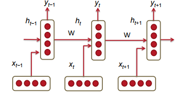 source: cs224 at stanford lecture notes, [4]
The inputs $x_i$ are individual vectors representing each word. Each node in the RNN takes two inputs, $x_i$ which represents the input of the $i$th word vector, and $h_{i-1}$ which represents the output from the $i-1$th node. The nodes in tern generate two outputs, $y_i$ and $h_i$, where $h_i$ is than fed in as an input to the next node. The nodes furthermore all share the same matrices, $W_{hh}$, $W_{xh}$, and $W_S$, which are used to generate the outputs.
- $y_i = \text{softmax}(W_Sh_i)$
- $h_i = \sigma(W_{hh}h_{i-1}+W_{hx}x_i) $
where $\sigma$ is the sigmoid function. The benefit from a neural network like this is that the output of the $i$th node depends not just on $x_i$ but also on $x_{i-1}$, $x_{i-2}$ and so on. For sentence processing, the steps are as follows:
- The words are encoded as vectors in a $D_w$ space, transforming an $n$ word sentence into a $n\times D_w$ tensor.
- The sentence is then transformed into a length $n_s$ vector by feeding the sentence words into a RNN, where each output is a $n_{s}$ vector. I will take the last output of the RNN (which depends on all words in the RNN) to be the sentence vector.
- I will add in one additional layer to the neural network to map from $n_s$ to $n_c$ where $n_c$ is the number of possible predicted labels (in this case 2).
- I will train this neural network using gradient descent.
I will construct this operation by using the popular library, tensorflow, to build the recurrent neural network, and gensim, to encode the word vectors. Tensorflow is an open source package written in optimized c++ and python, which can be used to build fast neural networks.
Word encodings 
To encode the words as vectors, I will use the gensim library and its word2vec encoder. The word2vec encoder I will use in this case determines the embeddings of a word by considering what words often occur near that word. For example, if president and prime minister occurred often together, the resulting vectors in the embedding would also appear close together. However, the word 'president' and the word 'prime-rib' would appear distant. The word2vec is a useful encoder since it also can preserve analogies. For example, the vector that points from man to king, is nearly the same as the vector that points from woman to queen, and the vector that points from cow to beef will be nearly the same as the vector that points from sheep to mutton.
To simplify the words more, I will first use a porter tokenizer to stem and tokenize all words before creating word embeddings. This will reduce the noise associated with our small sample size.
from gensim.models import Word2Vec
format_sentence, port_tokenizer
def process_data(X,y,embedding_dim=10,sentence_length=10):
    """Loads the text data and processes it into a padded array, and returns
    the array along with sentence lengths

    Parameters:
    --------------
    X: iterable array, shape = [n_samples,]
        entries consist of unprocessed sentences (i.e. text)
    y: iterable array, shape = [n_samples],
        entries consist of 0 or 1
    embedding_dim: int, default 10: the size of word vectors in the model
    sentence_length: int, default 10: the maximum sentence length to consider,
                     longer sentences will be shortened

    Returns:
    tuple consisting of X,y,length
    X: array, shape = [n_samples,sentence_length,embedding_dim]
    y: array, shape = [n_samples,2]
    length:, array, shape = [n_samples]
    """
    if(type(X)!=type(pd.Series())):
        X = pd.Series(X)
    if(type(y)!=type(pd.Series())):
        y =pd.Series(y)
    X = X.apply(format_sentence)
    X = X.apply(port_tokenizer)
    wv=Word2Vec(X,size=embedding_dim).wv
    X = X.apply(lambda ls:[list(wv[word]) for word in ls if
                                              word in wv.vocab])
    lengths = X.apply(lambda x:len(x) if len(x)<sentence_length else sentence_length)
    pad = [0. for i in range(embedding_dim)]
    X = X.apply(lambda ls:[ls[i] if i<len(ls) else pad for i in range(sentence_length)])
    X = X[lengths>0]
    y = y[lengths>0]
    lengths = lengths[lengths>0]
    #One hot encode y as [ham, spam]
    y = y.apply(lambda x:[0,1] if x else [1,0])
    return list(X),list(y),list(lengths)
Recurrent Neural Networks: 
The diagram for the network is shown below. 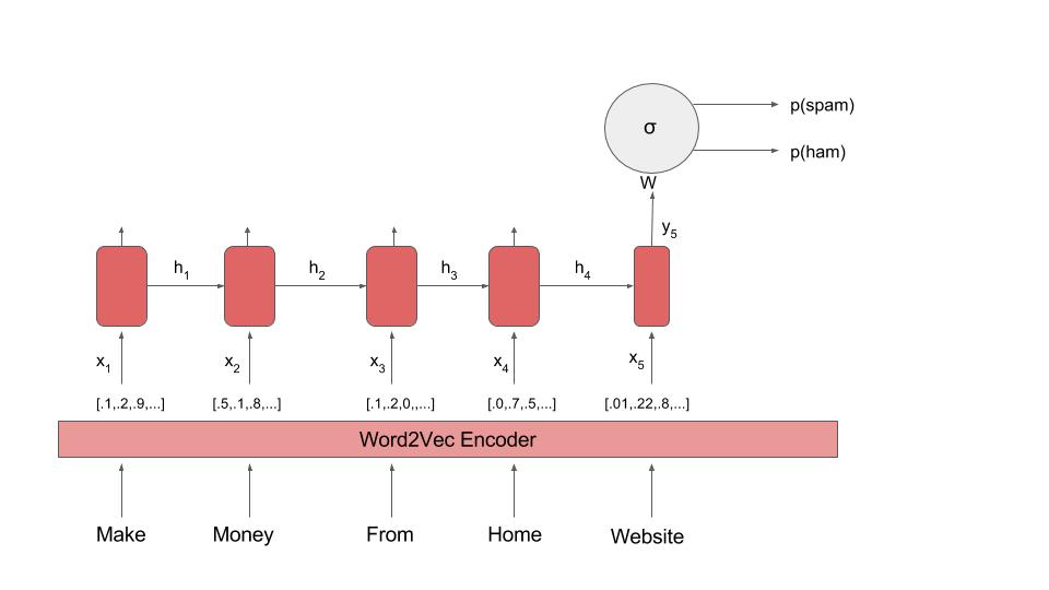
In tensorflow’s implementation of a simple RNN Cell, the outputs $y_i$ and $h_i$ are equal to each other, and are given by $$y_i=h_i = \text{activation}(V x_i + U h_{i-1} + b)$$ where $V$ and $U$ are matrices, and $b$ is the bias term. The activations of the output neurons $p(s)$ are then given by $$ p(s) = \text{softmax}(W\cdot h_l+b) $$ where $h_l$ is the last output from the rnn, and $W$ is a tensor. The predictions are made based on which class has the higher activation.
class Config():
    """ A class to hold the settings for neural network.
    """
    learning_rate=.005
    batch_size=100
    max_epochs=1000

    #length of word vectors
    n_input=20
    #max no of words per sentence
    n_steps=10
    n_classes=2
    #size of hidden RNN layer(i.e. length of sentence features)
    n_hidden=20
    #regularization parameter
    l2=.01

class RNN(BaseEstimator):
    """ A class for a simple variable length RNN to classify sentences.  The sentences
    must be preprocessed into arrays of word vectors prior to using the RNN.

    Parameters:
    -------------
    x_train: array, shape = [n_samples,n_steps,n_input]
        training data, n_steps refers to the number of words per sentence,
        n_input refers to the number of features per word.   Sentences smaller
        then n_steps must be padded with vectors to ensure each sample contains
        an array of the same size.

    x_test: array, shape = [n_samples,n_steps,n_input]
        test data, same conditions as apply to x_train

    y_train: array shape = [n_samples,n_classes]
        test data.  The data must be in the form of one hot vectors for each
        predicted class

    y_test: array shape = [n_samples,n_classes]
        test data, same conditions as apply to y_train

    length_train: int array or list, shape = [n_samples]
        The length of each training sentence before padding.

    length_test: int array or list, shape = [n_samples]
        The lengths of each test sentence before padding

    self.config: object which holds configuration parameters
        config.learning rate: float, default: .001
            The learning rate used in minibatch stochastic gradient descent
        config.batch_size: int, default: 100
            The size of minibatches fed into the NN for training.
        config.max_epochs: int, default: 50
            number of times to iterate over the training data for stochastic gradient descent
        config.n_input: int, default: 10
            length of embedding vectors for words
        config.n_steps: int, default: 10
            maximum number of words per sentence
        config.n_classes: int default: 2
            number of classes to predict
        config.n_hidden: int, default=10,
            size of vectors in RNN, represents the number of features per sentence
    """
    def __init__(self,config,cell_type='rnn'):
        self.config=config
        self.cell_type=cell_type

    def add_placeholders(self):
        """Initializes the placeholders to be used in the calculation"""
        n_steps = self.config.n_steps
        n_input = self.config.n_input
        n_classes = self.config.n_classes

        self.x_input = tf.placeholder(tf.float32,shape=[None,n_steps,n_input])
        self.y_input  = tf.placeholder(tf.float32,shape=[None,n_classes])
        self.length_input = tf.placeholder(tf.int32,shape=[None])

    def get_batch(self,i,X,y,lengths):
        """ returns the ith mini-batch of the training data
        Parameters:
        -------------
        i: int, which batch of training data to return
        X: arraylike, shape = [n_samples,n_steps,n_input]
            The training data
        y: arraylike, int, shape = [n_samples,n_classes]
            the class labels
        lengths: arraylike, int, shape = [n_samples]
            the lengths of each encoded sentence before
            padding is added

        Returns:
        --------------
        tuple consisting of batches for X,y, and length
        """
        batch_size = self.config.batch_size
        return X[i*batch_size:(i+1)*batch_size],\
                 y[i*batch_size:(i+1)*batch_size],\
                  lengths[i*batch_size:(i+1)*batch_size]

    def initialize_variables(self):
        """ Initializes the variables to be used in the tensorflow graph.
        """
        n_hidden = self.config.n_hidden
        n_classes = self.config.n_classes

        with tf.variable_scope('RNN'):
            weights = tf.get_variable('W',shape=[n_hidden,n_classes])
            biases = tf.get_variable('b',shape=[n_classes])

    def predict(self,X,lengths,reuse_var=False):
        """returns the logits predicted for each sentence

        Parameters:
        ---------------
        X, arraylike, shape=[n_samples,n_steps,n_features]
            preprocessed sentence arrays
        lengths, arraylike, shape=[n_samples] list of words
            per sentence before padding is added

        Returns:
        --------------
        logits, arraylike, shape = [n_samples,n_classes]
            predicted logits for each class
        """
        n_steps = self.config.n_steps
        n_hidden = self.config.n_hidden
        with tf.variable_scope('RNN',reuse=reuse_var):
            if self.cell_type=='rnn':
                rnn_cell = tf.contrib.rnn.BasicRNNCell(n_hidden,reuse=reuse_var)
            elif self.cell_type=='lstm':
                rnn_cell = tf.contrib.rnn.BasicLSTMCell(n_hidden,reuse=reuse_var,forget_bias=.6)
            outputs,states = tf.nn.dynamic_rnn(rnn_cell,
                                sequence_length=lengths,inputs=X,
                                time_major=False,dtype=tf.float32)

        with tf.variable_scope('RNN',reuse=True):
            W = tf.get_variable('W')
            b = tf.get_variable('b')
        output_list = tf.unstack(outputs,n_steps,1)
        batch_size = tf.shape(outputs)[0]
        last_rnn_output = tf.gather_nd(outputs,tf.stack([tf.range(
            batch_size),lengths-1],axis=1))
        return tf.matmul(last_rnn_output,W)+b

    def get_cost(self,pred,y):
        cost=tf.reduce_mean(tf.nn.softmax_cross_entropy_with_logits(
                logits=pred,labels=y))
        return cost

    def optimize(self,pred,y):
        """Adds the optimization layer to the graph.

        Parameters:
        ---------------
        pred: arraylike, shape = [n_samples,n_classes]
            logits for predicted class labels
        y: arraylike, shape = [n_samples,n_classes]
            one hot vector corresponding to actual values.
        returns:
        ------------
        tuple consisting of cost and optimizer,
        cost: float, total cost associated with predictions and actual values,
            uses cross entropy to compute the cost.
        optimizer:
            Adam optimizer to reduce the cost.
        """
        cost = tf.reduce_mean(tf.nn.softmax_cross_entropy_with_logits(
            logits=pred,labels=y))
        with tf.variable_scope('RNN',reuse=True):
            cost += self.config.l2*tf.nn.l2_loss(tf.get_variable('W'))
        optimizer = tf.train.AdamOptimizer(learning_rate=self.config.\
                                           learning_rate).minimize(cost)
        return cost,optimizer


    def train(self,X,y,lengths,verbose=False):
        """Trains the neural network given a batch of training data (X,y,length)
        Parameters:
        --------------
        X: array, shape = [n_samples,n_steps,n_input]
            training data, n_steps refers to the number of words per sentence,
            n_input refers to the number of features per word.   Sentences smaller
            then n_steps must be padded with vectors to ensure each sample contains
            an array of the same size.

        y: array, shape = [n_samples,n_classes]
            test data.  The data must be in the form of one hot vectors for each
            predicted class

        length: array or list, int, shape = [n_samples]
            The length of each training sentence before padding.
        """
        self.add_placeholders()
        self.initialize_variables()
        logits = self.predict(self.x_input,self.length_input)
        cost,optimizer = self.optimize(logits,self.y_input)
        y_pred = tf.argmax(logits,1)
        labels  = tf.argmax(self.y_input,1)

        #Create streaming measurements to find accuracy, precision and recall
        with tf.name_scope('measurements'):
            precision,prec_update = tf.contrib.metrics.streaming_precision(y_pred,labels)
            recall,recall_update = tf.contrib.metrics.streaming_recall(y_pred,labels)
            accuracy,accuracy_update = tf.contrib.metrics.streaming_accuracy(y_pred,labels)
        #Store variables related to metrics in a list, which allows all measuremnt variables
        #to be reset
        stream_vars = [i for i in tf.local_variables() if i.name.split('/')[0] == 'measurements']
        reset_measurements = [tf.variables_initializer(stream_vars)]

        self.saver = tf.train.Saver()

        with tf.Session() as sess:
            sess.run(tf.global_variables_initializer())
            sess.run(tf.local_variables_initializer())

            for epoch in range(config.max_epochs):
                av_loss = []
                for i in range(len(X)//self.config.batch_size):
                    batch_x,batch_y,batch_length = self.get_batch(i,X,y,lengths)
                    fd = {self.x_input:batch_x,self.y_input:batch_y,
                          self.length_input:batch_length}
                    loss,*_ = sess.run((cost,optimizer,
                                        prec_update,recall_update,
                                        accuracy_update)
                                       ,feed_dict=fd)
                    av_loss.append(loss)
                loss = np.array(av_loss).mean()
                acc,p,r = sess.run((accuracy,precision,recall))
                sess.run(reset_measurements)
                f1_score = 2*p*r/(p+r)
                if verbose and epoch%100==0:
                    print("Epoch {}, Minibatch Loss={:.6f}, training accuracy={:.5f}, f1={:.5f}"\
                              .format(epoch,loss,acc,f1_score))
            self.saver.save(sess,'/temp/model.ckpt')

    def test(self,X,y,lengths):
        logits = self.predict(self.x_input,self.length_input,reuse_var=True)
        cost = self.get_cost(logits,self.y_input)

        y_pred = tf.argmax(logits,1)
        labels  = tf.argmax(self.y_input,1)

        precision,prec_update = tf.contrib.metrics.streaming_precision(y_pred,labels)
        recall,recall_update = tf.contrib.metrics.streaming_recall(y_pred,labels)
        accuracy,accuracy_update = tf.contrib.metrics.streaming_accuracy(y_pred,labels)

        with tf.Session() as sess:
            self.saver.restore(sess, "/temp/model.ckpt")
            print("Model restored.")
            sess.run(tf.local_variables_initializer())
            cost = sess.run(cost,feed_dict={self.x_input:X,
                                                    self.y_input:y,
                                                    self.length_input:lengths})
            sess.run((prec_update,recall_update,accuracy_update),feed_dict={self.x_input:X,
                                                    self.y_input:y,
                                                    self.length_input:lengths})
            acc,p,r = sess.run((accuracy,precision,recall))
            f1_score = 2*p*r/(p+r)
            print("Testing Loss={:.6f}, testing accuracy= {:.5f}, f1={:.5f} ".format(cost,acc,f1_score))
tf.reset_default_graph()
config = Config()
config.n_input = 50
config.n_hidden=50
rnn = RNN(config)
X,y,lengths = process_data(data.CONTENT,data.CLASS,embedding_dim =config.n_input)
X_train,X_test,y_train,y_test,lengths_train,lengths_test = \
        train_test_split(X,y,lengths,train_size=.8,random_state=2)
rnn.train(X_train,y_train,lengths_train,verbose=True)
rnn.test(X_test,y_test,lengths_test)
From this, we can see that a neural network can achieve an f1 score of .92 and .86 on the training and test set respectively. While this is substantially lower than the scores of the logistic regression classifier, it is close to the score of the naive Bayes classifier. We can also explore how modifying the size of the hidden layer (the number of features per sentence) affects the training and testing f1 score.
for n_hidden in [5,10,20,50]:
    tf.reset_default_graph()
    config = Config()
    config.n_input = 50
    config.n_hidden=n_hidden
    rnn = RNN(config)
    print('RNN cell, n_hidden = {}'.format(n_hidden))
    rnn.train(X_train,y_train,lengths_train,verbose=True)
    rnn.test(X_test,y_test,lengths_test)
Although the training scores increase as the number of features per sentence (n_hidden) is increased, the test f1 scores decrease as the number of features increase, which indicates that adding in more sentence features beyond 5 is causing the model to overfit the data. Thus given the current amount of data, there is no benefit to going beyond 5 features in the hidden layer.
%%html
Conclusions 
| model | training f1 | test f1 |
|---|---|---|
| logistic regression | .99 | .94 |
| naive Bayes | .94 | .88 |
| RNN | .87 | .85 |
In the case of spam classification of short sentences and a small corpus, the most effective classifier was the simplest, which was a logistic regression classifier trained on a bag of words model. The naive Bayes classifier performed slightly better then the neural network on the test set, however, their performances were comparable. Given the small amount of documents, it is not surprising that the most simple classifier performed the best.